Sorta Sharpe

sharpe ratio is a second-order approximation to a higher-order problem

Note: This post has a lot of formal definitions that are really just superfluous for the high level understanding of what I actually think is important. If you are able to understand what a CDF graph is, then that’s all you need to be able to understand this post and feel free to skip the calculus!

“What’s your sharpe?”

I think that this is a pretty common question to get for someone managing a book or fund or whatever. It is a helpful stat to have in the back of your head when trying to understand the return profile that someone is running, but in isolation it’s ~okay~ at best. For example, do you really care if someone runs a 50 sharpe book but it only returns a few thousand dollars? Probably not. I mean at that point it’s kinda just like congrats you made a few thousand dollars. If the scalability to a reasonable size isn’t there then it becomes meaningless especially because if you recall from my previous post¹, I (and you) shouldn’t really care about variance for tiny dollar amounts.

Okay so sharpe matters when you have a strategy when you put on size? Yes. But is a strictly higher sharpe better if the EV is the same? Well it can be; it depends. In order for me to continue, we need to go over stochastic dominance (it’s related).

Stochastic Dominance

Stochastic dominance² is a way to say that one lottery (or strategy/outcome) is strictly better than another without making any assumptions about utility, other than that a high level of wealth is preferable (an increasing utility function). So I guess unless you take Biggy Small’s lyrics literally, this should apply to you.

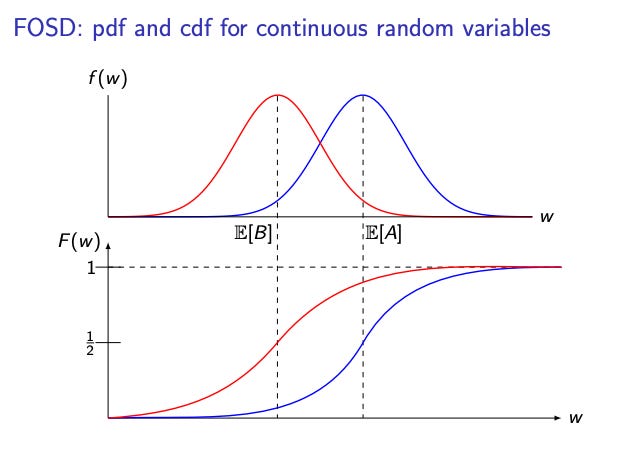
First Order Stochastic Dominance (FOSD)

As long as someone’s utility function is increasing w.r.t. wealth, then if one lottery (outcome) FOSDs another, it is preferred by all, regardless of the exact curvature of one’s utility function.

How do we know if one lottery FOSDs another? Well it is just that at every wealth level, the probability of ending up with less than or equal to that amount is never higher under the preferred lottery. In other words, the CDF of the preferred outcome is less than or equal to the CDF of the non preferred one at all points.

Below, A FOSDs B.

To be more precise with our definition:

\(\begin{aligned} \int_a^b u(w)\, \bigl[ f_{W_1}(w) - f_{W_2}(w) \bigr] \,dw &\ge 0 \end{aligned} \)

And now for some calculus II flashbacks, we will integrate by parts:

\(\begin{align*} &\int_a^b f'(x)\,g(x)\,dx \\ &\quad= f(b)g(b) - f(a)g(a) \\ &\qquad - \int_a^b f(x)\,g'(x)\,dx \end{align*} \)

\(\begin{aligned} g(w) &= u(w) \\ f'(w) &= f_{W_1}(w) - f_{W_2}(w) \\ f(w) &= F_{W_1}(w) - F_{W_2}(w) \end{aligned} \)

\(\begin{aligned} F_{W_i}(w) &= \int_{-\infty}^{w} f_{W_i}(t)\,dt \end{aligned} \)

\(\begin{aligned} F_{W_1}(a) &= F_{W_2}(a) = 0 \\ F_{W_1}(b) &= F_{W_2}(b) = 1 \end{aligned} \)

\(\begin{align*} &\int_a^b u(w)\,[f_{W_1}(w)-f_{W_2}(w)]\,dw \\ &\quad= u(b)\,[F_{W_1}(b)-F_{W_2}(b)] \\ &\qquad -\,u(a)\,[F_{W_1}(a)-F_{W_2}(a)] \\ &\qquad - \int_a^b u'(w)\,[F_{W_1}(w)-F_{W_2}(w)]\,dw \end{align*} \)

\(\begin{align*} &\int_a^b u(w)\,[f_{W_1}(w)-f_{W_2}(w)]\,dw \\ &\quad= - \int_a^b u'(w)\,[F_{W_1}(w)-F_{W_2}(w)]\,dw \end{align*} \)

\(\begin{aligned} \int_a^b u'(w)\, \bigl[ F_{W_2}(w) - F_{W_1}(w) \bigr] \,dw &\ge 0 \end{aligned} \)

\(\begin{aligned} F_{W_2}(w) - F_{W_1}(w) &\ge 0 \qquad \forall w \end{aligned} \)

\(\begin{aligned} \mathbb{E}[u(W_1)] &\ge \mathbb{E}[u(W_2)] \qquad \forall\ u'(w) > 0 \end{aligned} \)

\(\begin{aligned} \exists\, w_1, w_2 : \quad F_{W_1}(w_1) &> F_{W_2}(w_1), \\ F_{W_1}(w_2) &< F_{W_2}(w_2) \end{aligned} \)

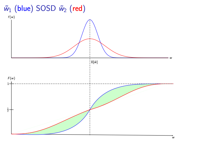
Second Order Stochastic Dominance (SOSD)

As long as a person’s utility function is increasing and concave in wealth (i.e., the person is risk-averse), if one lottery SOSDs another, it is preferred by all such individuals, regardless of the exact degree of risk aversion.

How do we know if one lottery SOSDs another? Unlike FOSD, this allows the distributions to cross (but only at one point!). At every wealth level, the area under the CDF of the preferred lottery is less than or equal to that of the non-preferred one. Equivalently, the cumulative probability of “bad outcomes,” when integrated over all thresholds, is always smaller. (It is worth noting that FOSD implies SOSD, but the reverse is not necessarily true.)

There can only be SOSD if the preferred lottery has an expected value greater than or equal to the non-preferred one. If the expected values are the same, then the preferred lottery must be a mean preserved spread of the non-preferred. In other words, the preferred lottery just has weakly lower higher order moments (variance, skew, and kurtosis). It is not enough to state that just because the variance is lower that a lottery SOSDs another (which is kind of my point with Sharpe that we will loop back to).

The integral condition:

\(\begin{align*} &S(w) = \int_a^w \bigl(F_{W_1}(s)-F_{W_2}(s)\bigr)\,ds \\ &\quad\ge 0 \qquad \forall\, w \in [a,b] \end{align*} \)

\(\begin{align*} &\mathbb{E}[W_1] = \mathbb{E}[W_2] \end{align*}\)

Difference in expected utilities:

\(\begin{align*} &\mathbb{E}[u(W_1)] - \mathbb{E}[u(W_2)] \\ &\quad= \int_a^b u(w)\,f_{W_1}(w)\,dw - \int_a^b u(w)\,f_{W_2}(w)\,dw \end{align*} \)

\(\begin{align*} &\quad= \int_a^b u(w)\, \bigl(f_{W_1}(w)-f_{W_2}(w)\bigr)\,dw \end{align*} \)

Integration by parts:

\(\begin{align*} &\int_a^b f'(x)\,g(x)\,dx \\ &\quad= f(b)g(b) - f(a)g(a) - \int_a^b f(x)\,g'(x)\,dx \end{align*} \)

\(\begin{align*} &g(w) = u(w) \end{align*} \)

\(\begin{align*} &f'(w) = f_{W_1}(w)-f_{W_2}(w) \end{align*} \)

\(\begin{align*} &f(w) = F_{W_1}(w)-F_{W_2}(w) \end{align*} \)

\(\begin{align*} &\int_a^b u(w)\, \bigl(f_{W_1}(w)-f_{W_2}(w)\bigr)\,dw \\ &\quad= \bigl[ u(w)\, \bigl(F_{W_1}(w)-F_{W_2}(w)\bigr) \bigr]_a^b \\ &\qquad - \int_a^b u'(w)\, \bigl(F_{W_1}(w)-F_{W_2}(w)\bigr)\,dw \end{align*} \)

Mean preservation means that the boundary term vanishes:

\(\begin{align*} &\mathbb{E}[W_1] = \mathbb{E}[W_2] \\ &\quad\Rightarrow \int_a^b \bigl(F_{W_1}(w)-F_{W_2}(w)\bigr)\,dw = 0 \end{align*} \)

\(\begin{align*} &\bigl[ u(w)\, \bigl(F_{W_1}(w)-F_{W_2}(w)\bigr) \bigr]_a^b = 0 \end{align*} \)

Reduced expression:

\(\begin{align*} &\mathbb{E}[u(W_1)] - \mathbb{E}[u(W_2)] \\ &\quad= - \int_a^b u'(w)\, \bigl(F_{W_1}(w)-F_{W_2}(w)\bigr)\,dw \end{align*} \)

Define cumulative CDF difference:

\(\begin{align*} &S(w) = \int_a^w \bigl(F_{W_1}(s)-F_{W_2}(s)\bigr)\,ds \end{align*} \)

\(\begin{align*} &S(a) = 0 \end{align*} \)

Integrate by parts (again!):

\(\begin{align*} &\int_a^b u'(w)\, \bigl(F_{W_1}(w)-F_{W_2}(w)\bigr)\,dw \\ &\quad= \bigl[u'(w)\,S(w)\bigr]_a^b - \int_a^b u''(w)\,S(w)\,dw \end{align*} \)

Final SOSD condition:

\(\begin{align*} &\mathbb{E}[u(W_1)] - \mathbb{E}[u(W_2)] \\ &\quad= \int_a^b \bigl(-u''(w)\bigr)\,S(w)\,dw \end{align*} \)

SOSD preference:

\(\begin{align*} &u'(w) > 0, \quad u''(w) \le 0, \quad S(w) \ge 0 \;\forall w \\ &\quad\Rightarrow\; \mathbb{E}[u(W_1)] \ge \mathbb{E}[u(W_2)] \end{align*} \)

Back to Sharpe

Ok, so we can probably see that if the expected value is substantially more, such that the CDFs never intersect, then the sharpe is irrelevant because we can have FOSD even under a lower sharpe ratio. When we have cases of equal mean and variance, higher order moments matter too.

Suppose that we have two lotteries with equal mean and variance, but switched skew:

\(\begin{array}{l} \textbf{Lottery A (positive skew)} \\[4pt] X \in \{-1 \text{ w.p. } 0.9,\; 9 \text{ w.p. } 0.1\} \\[4pt] \mathbb{E}[X] = (-1)(0.9) + 9(0.1) = 0 \\[4pt] \mathbb{E}[X^2] = (1)(0.9) + (81)(0.1) = 9 \\[4pt] \mathrm{Var}(X) = 9 \end{array} \)

\(\begin{array}{l} \textbf{Lottery B (negative skew)} \\[4pt] Y \in \{-9 \text{ w.p. } 0.1,\; 1 \text{ w.p. } 0.9\} \\[4pt] \mathbb{E}[Y] = (-9)(0.1) + 1(0.9) = 0 \\[4pt] \mathbb{E}[Y^2] = (81)(0.1) + (1)(0.9) = 9 \\[4pt] \mathrm{Var}(Y) = 9 \end{array} \)

Ok so clearly A and B have the same mean and variance but the skew is ‘flipped’. We should prefer lottery A under increasing, concave utility. I really like using extremes to highlight examples. Kelly Criterion never has you do anything with a chance of going to 0 since ln(0) → -inf (this is bad…lol). Suppose that you only have 9 dollars to your name, the negative skew can bring you to 0, where as the positive skew lottery cannot, so obviously we prefer A in that case, but even if we have more to our name, our preference should still be the same.

The Taylor expansion of ln(w) makes this a little more clear: +mean, -variance, +skew, -kurtosis, …

\(\begin{array}{l} f(w)=f(w_0) + f'(w_0)(w-w_0) + \dfrac{f''(w_0)}{2!}(w-w_0)^2 \\[6pt] \quad + \dfrac{f^{(3)}(w_0)}{3!}(w-w_0)^3 + \dfrac{f^{(4)}(w_0)}{4!}(w-w_0)^4 + \cdots \end{array} \)

\(\begin{array}{l} \mathbb{E}[\ln(W)] \approx \ln(\mathbb{E}[W]) - \dfrac{\mathrm{Var}(W)}{2\,\mathbb{E}[W]^2} + \dfrac{\mathbb{E}[(W-\mathbb{E}[W])^3]}{3\,\mathbb{E}[W]^3} - \cdots \end{array} \)

And this makes intuitive sense right? because if you look at a concave function, the left is ‘steeper’ than the right so moving equal distance to the left as the right has a bigger change in utility as the vertical distances you move are asymmetric.

And this is why even under two strategies, one having lower variance but the same mean (strictly higher sharpe) is not enough to let you know that you prefer the strategy with the higher sharpe. Perhaps the strategy with the higher sharpe has a rare, but nasty left tail, making the total expected utility less for risk-adverse individuals. The strategy must SOSD the other to be considered objectively better.

Sort of Vol Risk Premium (VRP)

Ok this is a little separate, but assume that options market makers (OMMs) are risk adverse individuals. Based on what we went over, where do you expect their fair value of the option w.r.t. the midpoint of the quotes that they show?

It must be below the midpoint as to be indifferent between a buy and a sell, the OMM needs to ask for strictly more edge on the ask to compensate for the fact that being short vol has negative skew for your payout, while as being long vol has positive skew. Therefore, they need ask for more edge to have added EV to compensate for the ‘reversed’ payout structure that drags down utility.

1.

2. Stochastic Dominance Wikipedia